The concept of a stable process is not new to the BIT service team. In the Kanban method, the definition of stability is not based on the (quite difficult) concept of assumption of stationarity but on the more intuitive notion that the arrival rate of new work items and the departure rate of completed work items are (in average) equals.
However, the bottom-line message is the same: if the process is not stable (under control), you cannot make forecasts.
Practically, it is possible to understand if the process is stable through the analysis of a chart: the Cumulative Flow Diagram (CFD).

The Cumulative Flow Diagram (CFD)

Its main purpose is to show you how stable your flow is and help you to understand where you need to focus on making your process more predictable. It gives you quantitative and qualitative insight into past and existing problems and can visualize massive amounts of data.
The “X” axis represents a timeline.
The “Y” axis is the actual (cumulative) number of the work items.

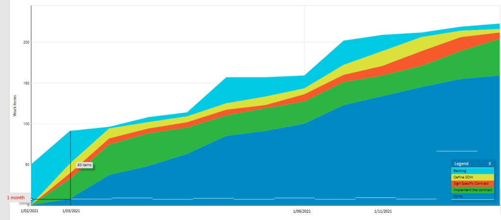
FIG 1 is the CFD of the Broker Activity workflow of BIT (Private & Public together).
The differently colored bands are the distinct stages of your work flow as they appear on the Kanban board itself.
The Kanban board visualizes the work flow; it is possible to say that it is a snapshot of the work flow in a specific moment. Analogously to the Statistical Process Control, it is necessary to have an analysis through the time line of the flow in order to apply useful analytics and charts.

Klaus Leopold (practical Kanban), explains that the goal should be that at least the gradients of Done and Committed run parallel; then the arrival rate (from Option Pool to Commited) and departure rate (from Commited to Done) are more or less equal.

Fig 2 shows exactly the state that should be attained with WIP limits: a stable work system. Such a perfectly stable system is rarely, if ever, seen in the real world.

In the Broker Activity Kanban board, the Commited flow of Fig 2 is composed by the Sign Specific contract and by the Implement flow (respectively: orange and green flow of Fig. 1).
So, the Commited Flow of fig 2 corresponds to the IN PROGRESS area of the Kanbanize board of the Broker Activity workflow of BIT.
The Option flow of Fig 2 corresponds to the Backlog and Requested Area of Fig 1.

For the Broker Activity workflow, this means that if we trace the line for Done and the line for the orange flow, they should contain only the colors of the stages that composes the area Done (blue) and In progress (orange and green).

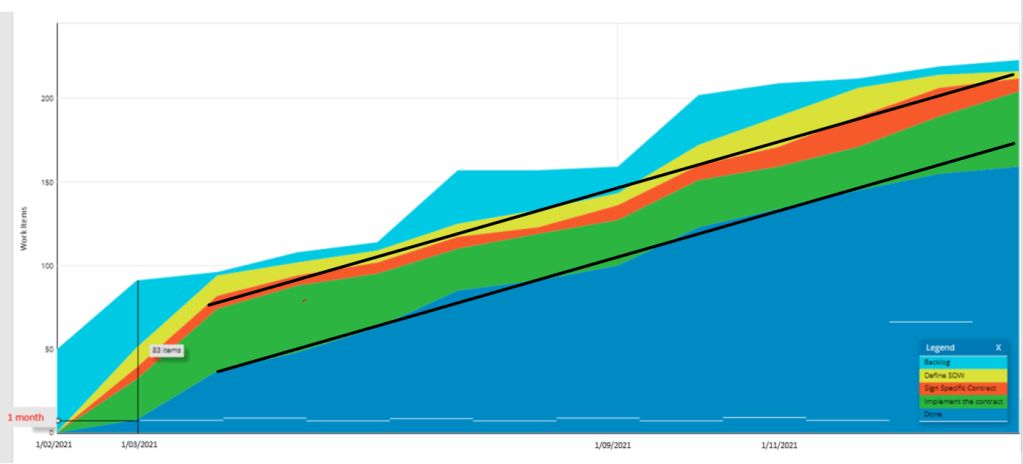
In Fig 3 the two first months are not considered for the stability analysis as the Kanban method was not yet fully implemented in the organization.

It is possible to say that the process looks quite stable.
In the period September-November it looks like the flow of Sign In Contract is narrowing; that means that the throughput of the stage it represents is higher than the entry rate. This is a sign that you’ve got more capacity than you really need at this stage, and you should relocate it to optimize the flow.
In the last month, it looks like the Implement the Contract flow is Widening. Whenever this happens on a cumulative flow diagram, the number of cards that enter the corresponding stage on the Kanban board is higher than the number of assignments leaving it. It is a common problem caused by multitasking and other waste activities that don’t generate value.

It is possible to note a strong peak for the months of July/August in the backlog flow; this peak was expected as every year there is a strong request of services from the public sector for that period. However, despite this seasonality, the system look stable; so the WIP limits are correctly defined to assure stability. It toosk to the system about two months to absorbe the pick in the backlog.

There is a second strong seasonality in the backlog flow in October/November (in this case originated from a seasonal pick of requests in the private and in the public sector). Also in this case it tooks to the system about two months to absorbe the pick in the backlog; however, as above mention, it looks that this second pick might have caused a wider flow in the Implementing to Contract.

The subject of seasonality was already brought to the attention of the management but the insight of this CFD can bring a further topic for the annual management review.

Cycle Time.

As workflow is (reasonable) stable, it is possible to use the CFD to (visually) have an idea of the (average) Cycle time.
The Cycle Time is the amount of time an item of work spends in the system. It is calculated from the moment that work starts (orange flow) until it is completed (blue flow).
As the CDF doesn’t follow the cycle time of each indvidual work item, the visualized cycle time is an average.
Fig 4 shows that in average a work item spent 3 months in the system.

Throughput

Throughput is the number of completed items of work in a given time frame.
The slope of that bottom line of Fig 3 shows the average throughput for the entiry time frame of the system.
In an (ideal) stable process, for any time frame you should obtain the same slop.
I agree that visually is not easy to have a quantitative feeling of the average throughpout. In this case, the “magic” formula of Fig. 6 might help.

Like for the Cycle time, this metric is average because not all of the tasks that have entered the stage necessarily leave it at the predetermined time frame. They might be moved to the next stage later in time.

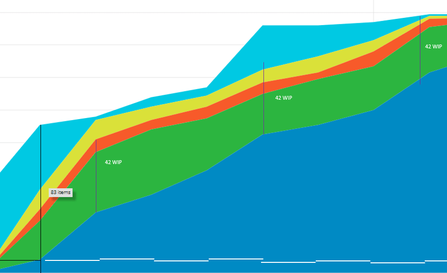
WIP (Work in Progress)

The diagram visualizes the number of work items that are in progress at each stage of your flow.
This can be measured using the vertical distance between the lines of each band.
Fig 5 shows the WIP of the Committed flow.
In an (ideal) stable process, this WIP should be a constant line.

I open a brief (I promise) analytic bracket for the “blue” audience of this post to represent the mathematical relationship of these 3 key measures:

Using the Little law equation, it is easy to calculate the (average) Throughput of the worfklow:
Throughput = WIP (58) / Cycle Time (3 months) = 19.3
In average, 19.3 Work items are completed in one month.

Going back to our visual approach of the stability, if you are still with me, I suggest this short but interesting video.